Homeownership remains a primary path to wealth accumulation for most Americans. For decades, as the economy has ebbed and flowed, the American dream of homeownership has been harder to come by for low-income households compared with wealthy households. But recently, buying a home has become more accessible to all income groups as the market has recovered.
As the U.S. copes with growing economic inequality, we examine where and why low-income households have ownership rates closer to that of wealthy households. Since homeownership rates vary from metro to metro, we measure homeownership inequality by the gap between the share of homeowners among the bottom third of households by income relative to the top third. Since retirees often own homes but don’t usually have incomes as high as during their working years, we’ve focused our attention on households headed by people considered to be prime working age (25 to 55 years).
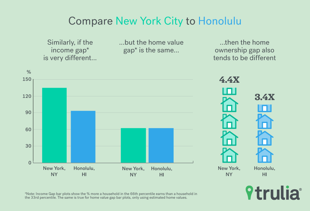
Since 1976, homeownership inequity has generally grown, but the chances of owning a home depend largely on the market. We found that in America’s biggest 100 housing markets, higher-income households tend to own their homes at as much as 4.4 times the rate of those at the bottom of the income ladder. But despite the national trend over the past few decades, not every housing market is off limits to low-income buyers. Things like the average age of a city’s population, the magnitude of a housing market’s price range, income inequality, and how long people stay in their homes all seem to play a role in ownership inequity.We found:
- Nationally, 77% of wealthy households own their own homes; almost 2.3 times the 34.9% homeownership rate of poor households. Since 2012, the ownership gap between high-income and low-income households has been trending downward, decreasing to 2.3 times from 2.4.
- Among the largest 100 metros, the homeownership gap is larger than it is nationally, with 79.3% of wealthy households now owning, which is 2.8 times higher than the 27.9% homeownership rate of poor households.
- Low-income households are more likely to own in metros such as Long Island, N.Y., Daytona Beach, Fla., and Troy, Mich., with wealthy households owning at less than 2 times the rate of their low-income peers.
- What determines the gaps? Homeownership inequality can’t be pinned to a single reason. Things like the range of household income, range of home prices, age of the population, and the proportion of the population that have lived in their home for less than five years all play a role, but none alone are strong predictors.

Homeownership Rates Rise With Rising Economic Tide
In the first half of 2017, the overall homeownership rate has ticked up after falling for last 10 years. This was partially a result of younger buyers, who often have low incomes, coming back into the market in greater numbers. The increase is largely in line with how economic cycles seem to play a role in rise and fall of homeownership rates, but not all recessions and expansions are created equal.
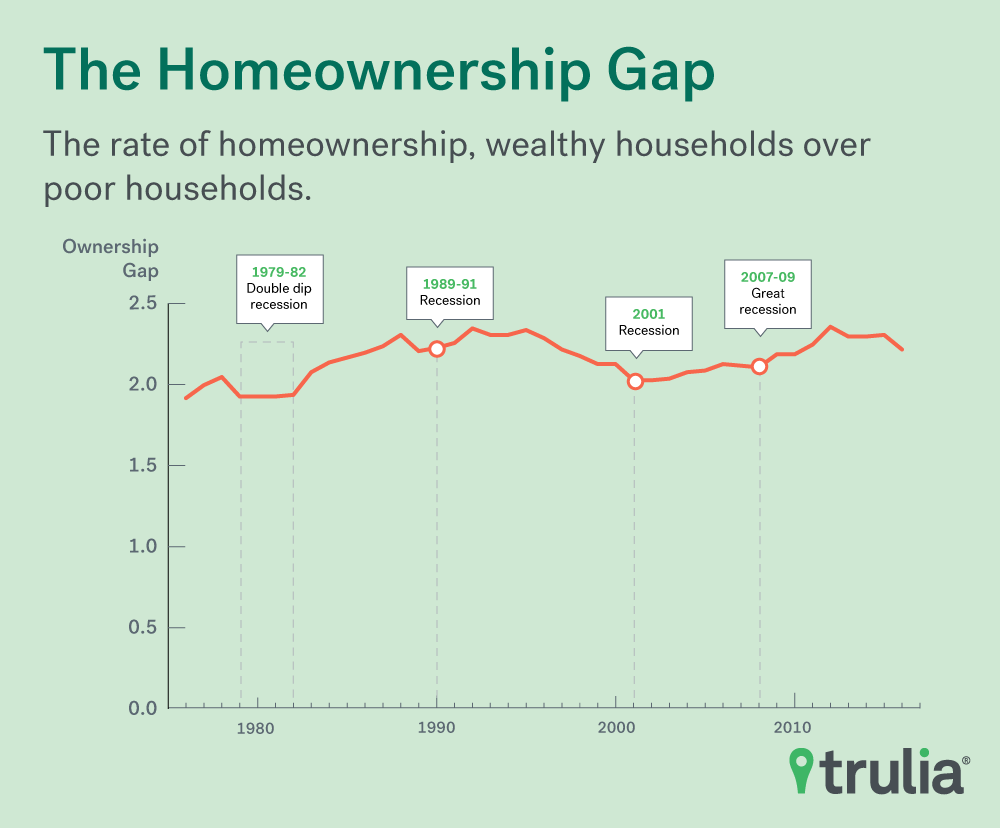
In 1976, affluent households owned at twice the rate of low-income households. Homeownership inequality grew rapidly during the ‘80s when the economy was expanding until the ‘89-‘91 recession. During this time, higher income households went from owning at 1.9 times the rate of low-income households in 1982 to 2.3 times the rate in 1988, shortly before the ’89-‘91 recession started. During the expansion between 1991 and 2001 though, the gap fell back down to 2.0. After the 2001 recession, the gap rose modestly before shooting back up again during the housing crisis and ensuing Great Recession.
During the Great Recession in the first half of the last decade (2007-2012), there was a dramatic increase in the homeownership gap between high-income households and low-income households. The housing and economic growth that has occurred during the recovery years has helped to narrow this gap. In many ways, our current economic expansion looks more like the expansion that took place in the ‘90s.
Larger Cities Feed Suburban Ownership Hotspots
Among the 100 largest metro areas, the housing markets with the highest overall homeownership rates include Long Island, Montgomery and Bucks counties in Pennsylvania, Camden, N.J., and Troy, Mich.,. Many of these places are smaller metros that are often located just outside of larger metros. Many have slightly older populations and serve partially as bedroom communities to big economic hubs.
Homeownership Inequality Highest in Northeast and West Coast
By comparison, housing markets with the widest homeownership gap are generally places with higher churn – people who move homes every five years or less –, little variation in home values, and higher income inequality. Markets that fit this bill include New Haven, Conn., New York, and Los Angeles, which have the biggest homeownership gaps at almost double the national rate.
The ownership gap between high- and low-income households generally seems to narrow as home values in a metro area become wider — up to a certain point. This could be because people of different income-levels are more likely to be able to find a suitable home to purchase in a place where the housing stock has more variation.
In Orange County, Calif., for example, where higher earning households are about 3 times more likely to own than low-income household, a home valued $700,960 (at the 66th percentile of all home) is only worth 41.5% more than a home in the 33rd percentile at $497,095. Working-age households in the 66th percentile by household income, or $108,393, make roughly twice as much, as those in the 33rd percentile of income at $49,961. In other words, less variation in home values means there are fewer opportunities for homeownership in price ranges that fall outside the norm for that area. These affects predominantly fall on low income households that are seeking out low-priced homes.

The opposite is true when looking at income inequality and how that relates to gaps in homeownership. There is a loose trend indicating that as the range between high- and low-income groups grows, so too does the gap in homeownership. As with home values though, this pattern only seems to hold to a certain point or in conjunction with other factors.

All the factors mentioned above explain only about 25% of the variation in the size of homeownership gaps between metros. Some of these factors though, such as home-value variation, have potential policy solutions, while others, especially those that are demographic-based, are largely outside the control of local governments. While demographic factors in some metros, such as a younger than average population, may be fueling unequal housing outcomes, along with a national trend that has been pointing to a gradually widening gap, there still seems to be plenty of opportunity for changes to local housing policy that could move the needle in a favorable way for low income groups.
Methodology
In looking at the ownership gap between high- and low-income households nationally, we used IPUMS micro-level CPS data going back to 1976 when the CPS began tracking ownership status. Only households headed by people between the ages of 25 and 55 were included in the analysis. Household income were grouped into low-, middle-, and upper-third categories and ownership rates were calculated from there.
For the metro-level analysis, 2015 5-year ACS micro-data was used, and similar filters and analysis were applied. Income groups were calculated and are unique for each metro though as opposed to applying the one national income category, since income sin one metro area can be very different from incomes in anther. The 33rd and 66th percentile home values were also incorporated into the data using internal price estimates.
A model to predict the size of the ownership gap in largest 200 metros was then built as follows:
Low-third/Upper-third ownership gap = income spread + (income spread)^2 + home value spread + (home value spread)^2 + Median Age + proportion living in home 5 years or less + (proportion living in home 5 years or less)^2
Sarah Flood, Miriam King, Steven Ruggles, and J. Robert Warren. Integrated Public Use Microdata Series, Current Population Survey: Version 4.0. 1976-2016. Minneapolis: University of Minnesota, 2015. http://doi.org/10.18128/D030.V4.0.
Steven Ruggles, Katie Genadek, Ronald Goeken, Josiah Grover, and Matthew Sobek. Integrated Public Use Microdata Series: Version 6.0 2015 5-year ACS. Minneapolis: University of Minnesota, 2015.


