America’s biggest housing markets are becoming more economically diverse neighborhood by neighborhood, a trend that’s not only an opportunity for potential buyers to break in but making those communities less homogenous.
But it’s not all necessarily good news. In most markets, the most affordable housing is disappearing.
Trulia studied home values as well as rental and owner-occupied[1] housing across the nation’s biggest metros. We found that during the last five years, expensive neighborhoods were still expensive when it came to affordability, but more moderately priced neighborhoods are on the rise.
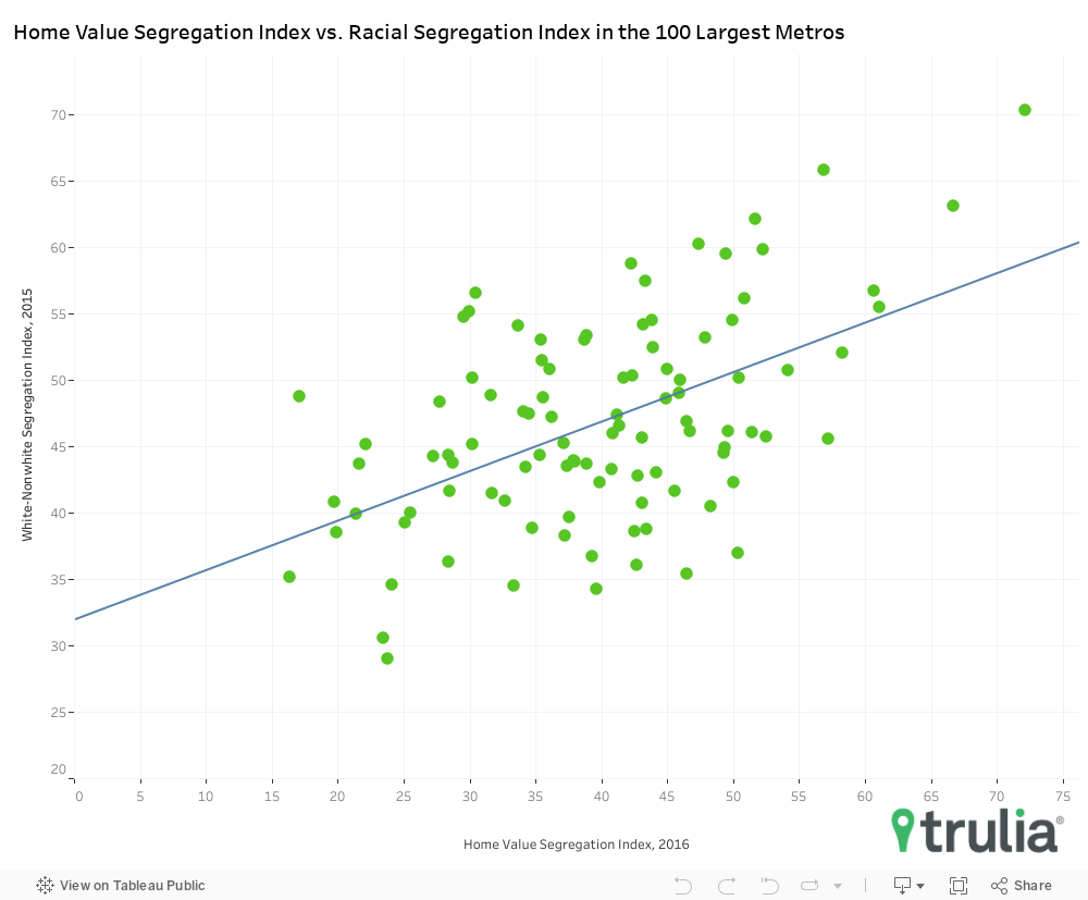
And, as part of our analysis, we noticed there’s a strong relationship between the unevenness of housing values across metros and the racial and income segregation within a metro.
That said, not every metro is seeing a widening gap. Some places – Phoenix and San Diego, for instance – saw the economic divide shrink. That means homebuyers and renters can find a mix of luxury and entry-level housing across those cities’ neighborhoods.
Why is this important? Identifying the economic disparities could be useful to those in charge of housing policy when it comes to persistent economic and racial segregation. For instance, local government could incentivize low-income housing programs in neighborhoods where lower-priced homes are disappearing.
To gauge the unevenness of housing values in a market we created an index that measures the share of neighborhoods[2] that contain housing in the lowest and highest tiers compared to the median price of a home in that metro.
Ƒor example, in the maps of Detroit, below, neighborhoods are ranked based on how far its median home value deviates from the metro’s median home value. Our index measures segregation of home values on a 100-point scale and reflects the share of neighborhoods in the very high value (dark orange) and very low value (dark green) category. The closer the index is to 100, the more segregated the metro is by home values. In 2016, for example, Detroit’s home value segregation index was 72.2, meaning that Detroit saw a high level of home value segregation with 72.2% of all neighborhoods falling into the most extreme value categories.
[1] We define owner-occupied housing to also include for sale or sold but not occupied homes.
[2] Neighborhoods are proxies for census tracts in this analysis.
We found:
- Nationally, House Hunters Have More Neighborhoods to Choose From:When it comes to home values across the 100 biggest metros, 1.62% of neighborhood housing[1] became less segregated in their respective regions from 2011 to 2016.
- Fifty-five out of the 100 biggest metros have fewer neighborhoods categorized as very low value than five years ago, an indication that the majority of these markets are recovering from the housing crisis.
- As Home Values Become More Polarized in a Market, Racial Segregation Increases: There is also a strong relationship between racial segregation in metros and housing values. Among the largest 100 metros, home-value segregation tends to increase as racial segregation increases.
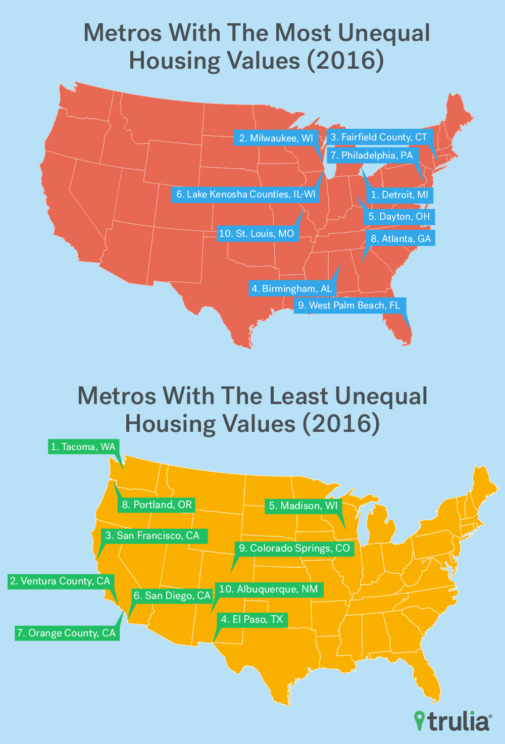
- Metros with the largest segregation of home values in 2016 were Detroit (72.2), Milwaukee (66.7), Fairfield County, Conn., (61.0), Birmingham, Ala., (60.6) and Dayton, Ohio, (58.3). While NOT a causation or correlation, Milwaukee and Detroit were incidentally also two of the most segregated cities in terms of black and white residents.
- Home Values Become Less Polarized Where the Sun Shines: In terms of changes in home value segregation Detroit, Charleston, S.C., and New York saw the largest increases from 2011 to 2016, while Phoenix, San Diego, and Cape Coral, Fla. saw the largest decreases.
- More Housing Segregation between Owners and Renters in Smaller Markets: There is a strong relationship between how big a metro is and the imbalance of rentals and owner-occupied homes. More populated metro areas tend to have a greater mix of rentals and owner-occupied housing across neighborhoods, while smaller metros are more likely to be segregated in terms of rental and owner-occupied homes.
[1] Metrics for the 100 largest metros are calculated as an average across all of these metros, weighted by the number of occupied housing units.
Across the 100 largest metros, the segregation of home values decreased by 1.62 index points from 2011 to 2016 while the segregation between rental and ownership units fell by a scant 0.06 index points. Likewise, there was a similar movement when it came to racial segregation. Segregation between white and black residents increased by nearly three index points (2.99) from 2010 to 2015 while segregation between white and non-white residents[1] fell by 0.42 index points.
The 5-year shift in home value segregation shows how much neighborhood home values can change. Since 2010 the U.S. housing market has been in a state of recovery after being hit with mass foreclosures, driving many neighborhoods to lose considerable value. Almost no change in the imbalance of rental and owner-occupied housing, however, reflects the relative immutability of rental and ownership opportunities, which only change only when significant amounts of construction occurs or when residences are converted into rental properties.
More than half (53) of the 100 largest metros saw decreases in home value segregation from 2011 to 2016. Far fewer metros experienced decreases in segregation of household income, just 36 out of 100 metros. The largest increases in home value segregation were in the Midwest and on the East Coast, while six of the 10 metros that reported the largest decreases were in California. The question is, how do changes in home value segregation impact the lowest and highest value neighborhoods?
It turns out that the metros that saw the largest increases in home value segregation mostly saw the proportion of the inexpensive neighborhoods increase, except for New York, Allentown, Pa., and Boston. In other words, metros with the largest increases in home value segregation actually saw the gap between the most and least expensive homes grow at the bottom end of the market. In other words, the share of least-expensive neighborhoods grew.
[1] White and black residents include white and black alone, non-Hispanic. Non-white persons include people of all non-white races alone plus people of Hispanic origin, regardless of race.
Metros with the Largest Increase in Home Value Segregation
| Home Value Segregation Index 2011 | Home Value Segregation Index 2016 | Difference in Home Value Segregation Index, 2011 to 2016 | Percentage Point Change in Share of Very Low Value Neighborhoods | Percentage Point Change in Share of Very High Value Neighborhoods | |
| Detroit | 49.9 | 72.2 | 22.29 | 17.37 | 4.92 |
| Charleston, S.C. | 38.1 | 50.3 | 12.24 | 10.08 | 2.16 |
| New York | 38.1 | 49.4 | 11.33 | 1.81 | 9.52 |
| Greensboro, N.C. | 30.5 | 41.4 | 10.83 | 11.77 | -0.94 |
| Wichita, Kan. | 40.3 | 49.3 | 8.96 | 8.96 | 0.00 |
| Milwaukee | 58.9 | 66.7 | 7.82 | 7.24 | 0.57 |
| Albany, N.Y. | 28.0 | 34.5 | 6.48 | 4.97 | 1.51 |
| Birmingham, Ala. | 54.6 | 60.6 | 6.09 | 6.20 | -0.10 |
| Allentown, Pa. | 28.3 | 34.1 | 5.79 | 1.97 | 3.82 |
| Boston | 24.6 | 30.0 | 5.40 | -1.62 | 7.02 |
On the other hand, metros with the largest decrease in home value segregation lost larger shares of least valuable neighborhoods than the most valuable neighborhoods. This suggests that metros with decreasing segregation, particularly in terms of fewer least valuable neighborhoods are rebounding from the housing crisis and experiencing a convergence of home values. During the housing crisis, concentrated foreclosures decimated home values in the lowest and lower- middle price tiers, but now that these units are back in the market, home values are recovering in the hardest hit neighborhoods.
| Home Value Segregation Index 2011 | Home Value Segregation Index 2016 | Difference in Home Value Segregation Index, 2011 to 2016 | Percentage Point Change in Share of Very Low Value Neighborhoods | Percentage Point Change in Share of Very High Value Neighborhoods | |
| Phoenix | 56.34 | 35.28 | -21.07 | -14.14 | -6.92 |
| San Diego | 39.19 | 21.64 | -17.55 | -14.23 | -3.32 |
| Cape Coral, Fla. | 64.75 | 49.34 | -15.41 | -10.81 | -4.6 |
| Sacramento, Calif. | 43.36 | 28.48 | -14.89 | -9.65 | -5.24 |
| Oakland, Calif. | 48.87 | 34.21 | -14.66 | -8.37 | -6.28 |
| Riverside, Calif. | 38.73 | 25.50 | -13.23 | -7.62 | -5.62 |
| Denver | 41.34 | 28.73 | -12.61 | -7.61 | -4.99 |
| Ventura County, Calif. | 29.19 | 17.11 | -12.08 | -8.22 | -3.86 |
| Bakersfield, Calif. | 43.14 | 31.61 | -11.54 | -8.52 | -3.01 |
| Deltona-Daytona Beach, Fla | 45.57 | 34.77 | -10.79 | -7.26 | -3.53 |
Measures of segregation of the housing market are related to racial and income segregation as well as the size of a metro’s population. The link between measures of home values and racial or income segregation are particularly revealing and may help to explain persistent residential segregation. Markets that are more segregated by housing values tend to also be more segregated in terms of household income and white-nonwhite residents. Meanwhile, there is a strong negative relationship between the segregation of rental and owner-occupied housing and a metro’s size by population. In other words, bigger metros tend to be less segregated by homes that are owned versus rented, and smaller metros more segregated.
These relationships suggest that efforts to decrease racial and income segregation, respectively, could be addressed by expanding choices in the housing market. The lack of housing diversity by price and ownership type constrain home seekers, particularly those that are lower income or those unable to purchase a home. As a result, they are relegated to finding homes where they are available, further entrenching both racial segregation and income segregation.
Methodology
Segregation indices reported here are calculated using two methods. The first is the Index of Dissimilarity (DI), which is used to measure how evenly distributed distinct groups are across census tracts in a given metro. The DI reports the share of one group that would need to move to another census tract in order to achieve the same makeup of the larger metro, and can take on values from 0 to 100. For example, a DI of 55 for white-black segregation in a metro would mean that 55% of either group would need to move to another census tract for that metro to become fully integrated. This measure is appropriate when comparing non-continuous groups and is applied here when discussing rental and ownership housing as well as race. The general formula can be found here:

Where i is the ith census tract in a metro area, p is the share of group 1 or 2 in a census tract, P is the share of group 1 or 2 in the entire metro.
The second is the Index of Proportional Distribution (PI) used for continuous measures such as income or home values. This index counts of the number of census tracts that fall in one of six buckets based on the ratio of the median value of the metric in question at the census tract level to that of the larger metro. The PI is the share of census tracts that fall in the extreme bottom and top buckets, or categories 1) and 6) defined below. For example, if a metro has 100 census tracts and 40 census tracts have very low home values and 20 have very high homes relative to the median home values in the metro, the PI would be 40. The ratios that define the six categories used here are: 1) very low value – under 0.67; 2) low value – 0.67 to 0.8; 3) low-medium value – 0.8 to 1.0; 4) high-medium value – 1.0 to 1.25; 5) high value – 1.25 to 1.5; and 6) very high value – 1.5 and above.
Data on race, ownership type of housing units and income are from the U.S. Census’ 5-Year American Community Survey from 2010 and 2015. Figures from these surveys represent a rolling average over five-year periods ending in the year of release. The choice of using five-year data was driven by the fact that samples are large enough to cover census tracts. Note that because the ACS is a sample survey, they are subject to margins of error. Rental housing is defined by both occupied rental housing units as well as vacant housing that is on the rental market (e.g. rented but not occupied and or for-rent but not occupied). Ownership housing includes occupied owned housing units as well as vacant units that cannot be rented (e.g. sold but not occupied, for-sale but not occupied, and vacant homes used as second homes).