UPDATED 7/22 1:50 ET: This report has been updated to correct price-change data from a proprietary source to government data (FHFA).
- Builders are providing less housing now as prices rise than they have in the past.
- Many places in the Southwest and Southeast actually provide ample new housing units when demand rises, but others in the Pacific West and Northeast don’t.
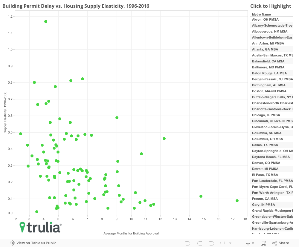
- For every month delay in approving new building permits, a housing market’s ability to meet housing demand falters
Why do some places struggle with a lack of housing while others seem to have too much?
During the last two decades San Francisco and Pittsburgh have been stingy when it comes to homebuilding and prices have risen. Contrast those metros with Las Vegas and Atlanta, some of the biggest foreclosure casualties in the housing crisis.
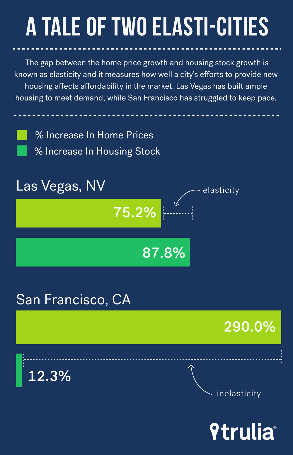
We studied the rate of homebuilding and the market prices for the nation’s biggest metros during the last 20 years to determine how housing policy affected what we economists call “elasticity” – simply put: how much new housing is built relative to demand. Markets with greater elasticity build more housing relative to price changes than markets with lower elasticity.
We found that the rate at which the nation’s housing stock has grown relative to demand is low and that while elasticity has fluctuated during the last 30 years, builders are providing less housing now as prices rise than they have in the past.
Of late, land use regulation, and in particular, zoning, has been blamed for keeping supply low in many markets. That story, however, is a simplistic one that overlooks the nuances involved with how local governments actually employ zoning across the country. Our research finds that local bureaucracy, measured by building approval delays, affect housing supply elasticity rather than restrictive zoning. Our other findings – and keep in mind that the higher the elasticity number, the more housing is built to meet demand – include:
- Nationally, long-run housing supply elasticity is at 0.17, three points below the 30-year average of 0.2, and just over half of peak elasticity of 0.29 in 1999Q4.
- Long-run elasticity at the metropolitan level varies substantially, from over 0.8 in Las Vegas, Raleigh-Durham-Chapel Hill, N.C., and Albuquerque, N.M., to under 0.05 in San Francisco, Los Angeles, and New Orleans.
- Local bureaucracy, rather than zoning, accounts for much of the difference in long-run supply elasticity across the country. For every month delay in approving new building permits, long-run supply elasticity drops by .03. We also find no statistically significant evidence that restrictive zoning reduces elasticity.
How Supply Elastic are U.S. Housing Markets?
How much the housing stock changes relative to prices – called supply elasticity by economic wonks – is an important metric of housing market health. For perspective, a value of one indicates that a one percent increase in housing price is associated with a one percent increase in the housing stock over a given time period. Both natural restrictions as well as government regulation can affect how elastic a given market is. For example, it is naturally much more difficult to build new homes in places with steep topography surrounded by water – such as San Francisco – than it is in areas with a flat buildable landscape, like Phoenix. It is also easier to get approval for new development in areas with less regulation, such as New Orleans and Mobile, Ala., than it is in areas with more regulation, like Honolulu and Los Angeles. In this report, we take a look at how much the housing stock is expanding relative to demand nationally and in the 100 largest markets. We also estimate the relative impact of different types of land use regulation – as measured by the Wharton Residential Land Use Regulation Index (WRLURI) from the University of Pennsylvania – on housing market elasticity.
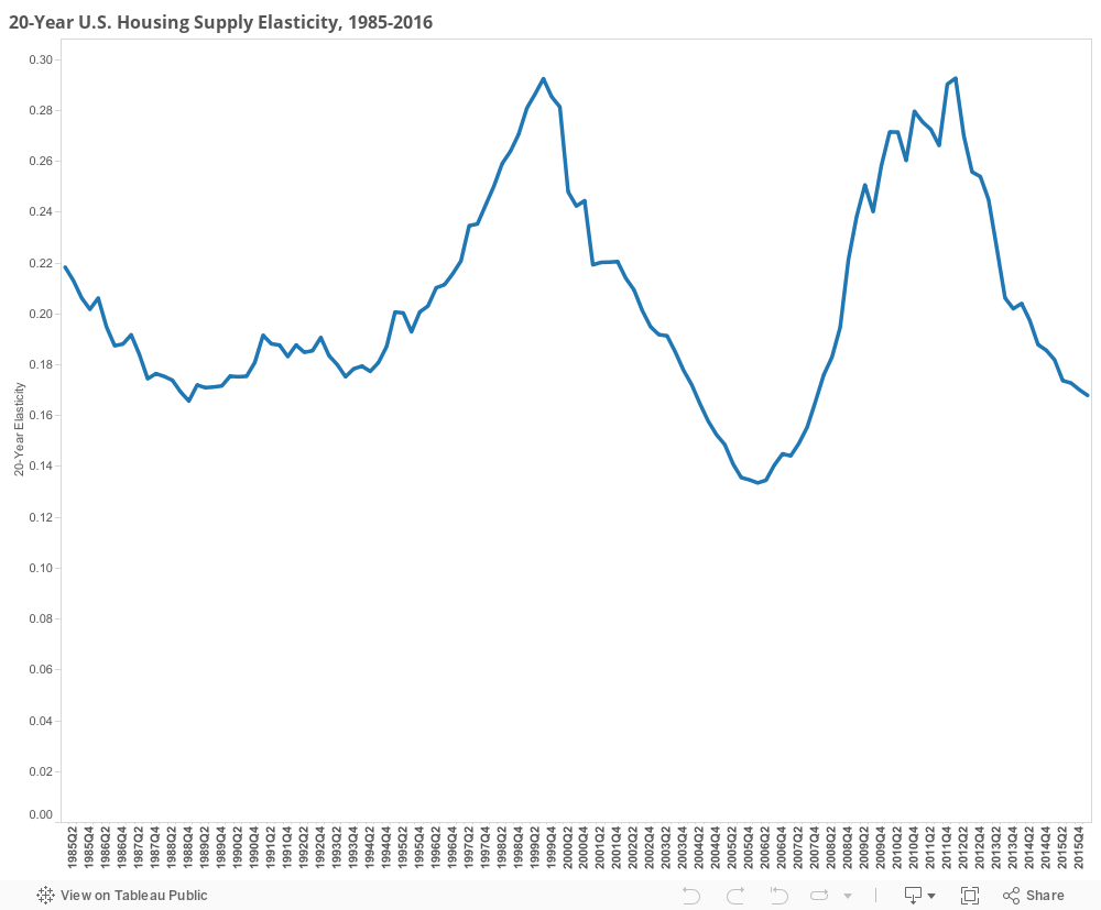
Over the last 30 years, long-run supply elasticity for the nation has fluctuated between 0.13 and 0.29. As of 2016Q1, that number was at a 0.17, down from 0.18 last year. So as a country, we are providing fewer new housing units as prices rise than we have in the past. Of course, the U.S. housing market is really a collection of individual metropolitan markets, and we find that elasticity varies considerably among them.
| U.S. Metro | % Increase in Housing Stock, 1996-2016 | % Increase in Housing Prices, 1996-2016 | Housing Supply Elasticity, 1996-2016 |
|---|---|---|---|
| Las Vegas, NV | 87.8% | 75.2% | 1.17 |
| Raleigh-Durham-Chapel Hill, NC | 71.6% | 87.2% | 0.82 |
| Albuquerque, NM | 37.5% | 46.1% | 0.81 |
| Charlotte-Gastonia-Rock Hill, NC-SC | 60.9% | 76.1% | 0.80 |
| Atlanta, GA | 53.4% | 68.9% | 0.77 |
| Indianapolis, IN | 30.4% | 44.3% | 0.69 |
| Columbia, SC | 44.7% | 66.4% | 0.67 |
| Greensboro–Winston Salem–High Point, NC | 31.4% | 47.0% | 0.67 |
| Washington, DC | 78.0% | 132.5% | 0.59 |
| Fort Myers-Cape Coral, FL | 73.4% | 126.2% | 0.58 |
| NOTE: Among the 100 largest U.S. metro areas, full data available here. (This chart was updated 7/22 1:50 pm ET to include FHFA price data) | |||
Of the 100 largest metros, Las Vegas has been the most elastic housing market in the U.S. over the past 20 years. Prices over this period have increased there 75.2%, but the housing stock increased 87.8%, leading to an elasticity estimate of 1.17. Other relatively elastic markets in the U.S. include Raleigh-Durham-Chapel Hill, Albuquerque, Charlotte and Atlanta where supply elasticity ranges from 0.77 to 0.82.
| U.S. Metro | % Increase in Housing Stock, 1996-2016 | % Increase in Housing Prices, 1996-2016 | Housing Supply Elasticity, 1996-2016 |
|---|---|---|---|
| New Orleans, LA | 1.7% | 80.7% | 0.02 |
| Pittsburgh, PA | 3.9% | 99.0% | 0.04 |
| Los Angeles-Long Beach, CA | 8.6% | 210.8% | 0.04 |
| San Francisco, CA | 12.3% | 290.0% | 0.04 |
| Buffalo-Niagara Falls, NY | 3.3% | 76.3% | 0.04 |
| Scranton–Wilkes-Barre–Hazleton, PA | 4.7% | 85.4% | 0.05 |
| New York, NY | 10.9% | 188.3% | 0.06 |
| Long Island, NY | 8.5% | 130.8% | 0.06 |
| Springfield, MA | 6.1% | 92.5% | 0.07 |
| San Jose, CA | 19.5% | 295.1% | 0.07 |
| NOTE: Among the 100 largest U.S. metro areas, full data available here. (This chart was updated 7/22 1:50 pm ET to include FHFA price data) | |||
On the other hand, there are many markets where elasticity is low. New Orleans tops the list of least elastic housing markets, where house prices have increased by 80.7% over the past 20 years but the housing stock only increased 1.7%. While New Orleans has the lowest elasticity in the U.S., much of the reason is due to major the major loss of housing that occurred in the city from Hurricane Katrina. In addition, low elasticity isn’t much of a problem in other markets that have low elasticity, such as Buffalo and Scranton, Pa., as several of these have vacancy rates of 10% or more.
Taking into account vacancy rates are important when determining whether low elasticity is a problem in a given market, as a lot of empty new homes allows new demand to be absorbed into the vacant units and without the need for new ones. On the other hand, low elasticity is a problem in other markets that make the bottom of the the list. In some of these markets – such as Los Angeles, San Francisco, and San Jose – home prices have tripled over the past twenty years, and affordability has fallen dramatically. For example, in San Jose – with an estimated elasticity of just 0.07 – middle class households have to spend about 13% more of their income to the median priced home compared to just four years ago, so supply is not keeping up enough to moderate affordability.
Blame Bureaucracy, Not Zoning, for Reducing Elasticity
A natural question to ask: why are some markets more elastic than others? Much academic and industry research recently has targeted restrictive zoning as the culprit in preventing enough new supply from coming onto the market. After all, building 100 new homes on a lot is difficult to do if it is only zoned for 50. However, zoning is not always a binding constraint. Most local governments allow for landowners and/or developers to apply for a zoning change that would allow more units to be built than the existing zoning code allows. While costlier and more time consuming for land developers, a zoning change can theoretically allow zoning to more closely follow the market. In the example above, a developer might apply for a zoning change to allow for 100 units, but settle on 75 after consultation with local authorities and neighbors. The downside to pursuing a zoning change is that in some circumstances it can take several months or years to successfully navigate, which in turn, adds more cost and risk to a project. As costs and risk associated with a housing development increases, so too does the likelihood that it will be scaled down or not completed at all.
In fact, we find that metros with longer administrative delays in rezoning and lot approvals are strongly correlated with lower long-run housing supply elasticity than metro with fewer delays, while restrictive zoning is not. See methodology section below for detail of our analysis, which includes regression modeling of the WRLURI components.
In sum, the rate at which we are providing housing in the U.S. relative to demand is low compared to historical standards, but this varies quite immensely across the largest 100 markets. Many places in the Southwest and Southeast actually provide a decent number of new housing units when demand rises, but others in the Pacific West and Northeast don’t. While it is tempting to blame the most popular tool of local land use regulation, zoning, we find that it is actually delays in the building permit approval process that affecting the ability of builders to meet demand. This is because zoning can formally be changed, while uncertainty over building approval cannot.
Methodology
To estimate long-run housing supply elasticity, we compare the 20-year change in a metro’s housing stock to the 20-year change in quality adjusted house prices. For estimates of the housing stock, we combine Moody’s Analytics estimates from 1970-2009 with Census Bureau’s Population Estimates Program (PEP) from 2010-2015, and extrapolate forward to 2016 using Census building permit data.
For price change estimates, we use FHFA repeat sales data from 1975-2016.
For measures of land use regulation, we use the 2008 Wharton Residential Land Use Regulatory Index (WRLURI) from the University of Pennsylvania, available for download and use here. The WRLURI is derived from a comprehensive survey of local governments across the U.S. on the types and performance of land regulation they employ. The WRLURI is composed of 11 sub-components that measure the restrictiveness of different types of regulatory measures. A brief description of each subcomponent is listed in the table below.
Using a simple regression analysis, we estimate the correlation of each regulatory measure indexed in the WRLURI (see table below for a description of each measure and regression results) with our estimate of housing supply elasticity across the 100 largest U.S. metros. While each regulatory measure is a subcomponent of the aggregate WLURI, only one – the approval delay index – is statistically significant in explaining why some metros have high elasticity and others are low. What’s more, regression analysis also controls for the intervening effect of other factors, so we can be sure that other measures in the index, such as restrictive zoning, are not confounding the result of approval delay. The impact is also relatively strong – each month of approval delay is correlated with a .03 decrease in housing supply elasticity. For example, over half of the -0.68 difference in supply elasticity between Honolulu (elasticity of 0.09) and Atlanta (elasticity of 0.77) can be explained by the difference in approval delays (13-month difference X -0.03 = -0.39). Surprisingly, one WRLURI measure most often blamed for stifling development – restrictive zoning – is not correlated at all with lower housing supply elasticity.
Much of the inspiration for this report comes from: Mayer, Christopher J., and C. Tsuriel Somerville. “Land use regulation and new construction.” Regional Science and Urban Economics 30.6 (2000): 639-662.
|
WRLURI Components and Regression Results |
||
| WRLURI Component | Component Description | Regression Estimate (Correlation with 20-Year Housing Supply Elasticity) |
| Local Political Pressure Index (LPPI) | Metro-wide measure of the influence of local groups | 0.07 |
| State Political Involvement Index (SPI) | Measure of state-wide influence in municipal land use regulation | -0.02 |
| State Court Involvement Index (SCII) | Measure of state-court deference to municipal regulations in land use cases. | 0.06 |
| Local Zoning Approval Index (LZAI) | Metro-wide measure of how many approving bodies must approve a project that requires a zoning change. | -0.01 |
| Local Project Approval Index (LPAI) | Metro-wide measure of how many approving bodies must approve a project that does not require a zoning change. | -0.04 |
| Local Assembly Index (LAI) | Metro-wide measure of whether there is a community meeting held in which any zoning or rezoning request must be presented and voted on. | -0.10 |
| Supply Restrictions Index (SRI) | Metro-wide measure of housing unit or permit constraints or caps. | -0.01 |
| Density Restrictions Index (DRI) | Metro-wide measure of the use of minimum lot size requirements. | 0.05 |
| Open Space Index (OPI) | Metro-wide measure of whether developers are required to provide or pay for open space. | 0.03 |
| Exactions Index (EI) | Metro-wide measure of whether developers are required to pay for infrastructure improvements. | -0.03 |
| Approval Delay Index (ADI) | Metro-wide weighted average number of months for residential permit approval | -0.03* |
| NOTE: Among the 100 largest U.S. metro areas, full data available here. Dependent variable in the regression is the 20-year estimate of housing supply elasticity. * indicates statistical significance at the .05 level. R2 for the regression model is 0.22. Regression coefficients can be interpreted as the change in elasticity for every unit change in the WRLURI component. | ||